Housing Prices in Recessions

Hypothesis Testing

Hypothesis: University towns have their mean housing prices less affected by recessions.

Background

A quarter is a specific three month period, Q1 is January through March, Q2 is April through June, Q3 is July through September, Q4 is October through December.
A recession is defined as starting with two consecutive quarters of GDP decline, and ending with two consecutive quarters of GDP growth.
A recession bottom is the quarter within a recession which had the lowest GDP. -A university town is a city which has a high percentage of university students compared to the total population of the city.
Hypothesis: University towns have their mean housing prices less effected by recessions. Run a t-test to compare the ratio of the mean price of houses in university towns the quarter before the recession starts compared to the recession bottom. (price_ratio=quarter_before_recession/recession_bottom)

The following data files are available for this assignment:

From the Zillow research data site there is housing data for the United States. In particular the datafile for all homes at a city level, City_Zhvi_AllHomes.csv, has median home sale prices at a fine grained level. From the Wikipedia page on college towns is a list of university towns in the United States which has been copy and pasted into the file university_towns.txt. From Bureau of Economic Analysis, US Department of Commerce, the GDP over time of the United States in current dollars (use the chained value in 2009 dollars), in quarterly intervals, in the file gdplev.xls. For this assignment, only look at GDP data from the first quarter of 2000 onward.

Previewing the Data

To get started, I uploaded the required libraries. The independent samples t-test is used in this case.

import pandas as pd
import numpy as np
from scipy.stats import ttest_ind

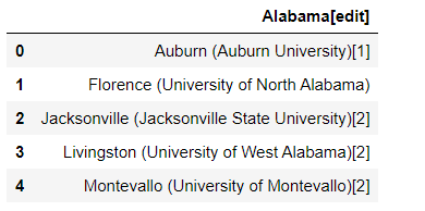
Let’s view the list of university towns.

df = pd.read_fwf('university_towns.txt')
df.head()

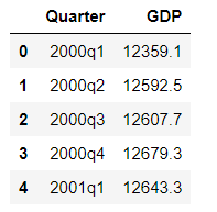
Now, let’s check out the US Department of Commerce GDP data.

GDP = pd.read_excel('gdplev.xls', usecols=[4,6], skiprows=219, names = ['Quarter', 'GDP'])
GDP['GDP'] = pd.to_numeric(GDP['GDP'])

GDP.head()

Finally, let’s look at our Zillow housing data.

zillow = pd.read_csv("City_Zhvi_AllHomes.csv")
zillow.head()

Cleaning the Data

First, I had to map states to acronyms to merge the university towns with the zillow dataset. So, I used this dictionary.

states = {'OH': 'Ohio', 'KY': 'Kentucky', 'AS': 'American Samoa', 'NV': 'Nevada', 'WY': 'Wyoming', 'NA': 'National', 'AL': 'Alabama', 'MD': 'Maryland', 'AK': 'Alaska', 'UT': 'Utah', 'OR': 'Oregon', 'MT': 'Montana', 'IL': 'Illinois', 'TN': 'Tennessee', 'DC': 'District of Columbia', 'VT': 'Vermont', 'ID': 'Idaho', 'AR': 'Arkansas', 'ME': 'Maine', 'WA': 'Washington', 'HI': 'Hawaii', 'WI': 'Wisconsin', 'MI': 'Michigan', 'IN': 'Indiana', 'NJ': 'New Jersey', 'AZ': 'Arizona', 'GU': 'Guam', 'MS': 'Mississippi', 'PR': 'Puerto Rico', 'NC': 'North Carolina', 'TX': 'Texas', 'SD': 'South Dakota', 'MP': 'Northern Mariana Islands', 'IA': 'Iowa', 'MO': 'Missouri', 'CT': 'Connecticut', 'WV': 'West Virginia', 'SC': 'South Carolina', 'LA': 'Louisiana', 'KS': 'Kansas', 'NY': 'New York', 'NE': 'Nebraska', 'OK': 'Oklahoma', 'FL': 'Florida', 'CA': 'California', 'CO': 'Colorado', 'PA': 'Pennsylvania', 'DE': 'Delaware', 'NM': 'New Mexico', 'RI': 'Rhode Island', 'MN': 'Minnesota', 'VI': 'Virgin Islands', 'NH': 'New Hampshire', 'MA': 'Massachusetts', 'GA': 'Georgia', 'ND': 'North Dakota', 'VA': 'Virginia'}

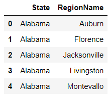
I cleaned the university_towns data to remove any weird characters.

def get_list_of_university_towns(): 

    with open('university_towns.txt', "r") as reader:
        lines = reader.readlines()
    reader.close()
    
    df = pd.DataFrame(columns=('State', 'RegionName'))
    count = 0
    state = ""
    region = ""
    
    for line in lines:
        line = line.rstrip('n')
        line = line.strip()
        if 'edit' in line:
            state = line.split('[')[0]
        else:
            region = line.split(' (',1)[0]
            df.loc[count] = [state, region]
            count = count + 1
    
    df.reset_index(inplace=True,drop=True)
    return df
    
get_list_of_university_towns()

Defining Quarters

Using the GDP data and the definition of a quarter as described in the background, I returned the quarter values with year in an easily usable string format when I found the start of the recession.

def get_recession_start():
#    '''Returns the year and quarter of the recession start time as a 
#    string value in a format such as 2005q3'''
    
    GDP = pd.read_excel('gdplev.xls', usecols=[4,6], skiprows=219, names = ['Quarter', 'GDP'])
    GDP['GDP'] = pd.to_numeric(GDP['GDP'])


    Quarter = []

    for i in range(len(GDP)-2):
        if ((GDP.iloc[i][1] > GDP.iloc[i+1][1]) & (GDP.iloc[i+1][1] > GDP.iloc[i+2][1])):
            Quarter.append(GDP.iloc[i+1][0])
            break
    return Quarter[0]
get_recession_start()

‘2008q3’

Next, I found the end of the recession.

def get_recession_end():
    start = get_recession_start()
    GDP = pd.read_excel('gdplev.xls', usecols=[4,6], skiprows=219, names = ['Quarter', 'GDP'])
    GDP['GDP'] = pd.to_numeric(GDP['GDP'])
    start_index = GDP[GDP['Quarter'] == start].index.tolist()[0]
    for i in range(start_index, len(GDP)-2):
        if ((GDP.iloc[i][1] < GDP.iloc[i+1][1]) & (GDP.iloc[i+1][1] < GDP.iloc[i+2][1])):   
            return GDP.iloc[i+2][0]
get_recession_end()

‘2009q4’

Finally, I found the bottom of the recession.

def get_recession_bottom():
    
    start= get_recession_start()
    end = get_recession_end()
    GDP = pd.read_excel('gdplev.xls', usecols=[4,6], skiprows=219, names = ['Quarter', 'GDP'])
    GDP['GDP'] = pd.to_numeric(GDP['GDP'])
    
    recession = GDP[(GDP['Quarter'] <= end) & (GDP['Quarter'] >= start)]
    recession.reset_index(inplace=True)
    recession.drop(['index'], axis=1, inplace=True)
    min_index = recession['GDP'].idxmin()
    return recession.iloc[min_index][0]
    
get_recession_bottom()

‘2009q2’

To use the quarterly values I created when finding the recession start/bottom/end, I had to convert the housing data to quarters as defined at the beginning and take the mean of the 3 months in the quarter.

def convert_housing_data_to_quarters():
    
    # Retrieved the housing data.
    df= pd.read_csv("City_Zhvi_AllHomes.csv")
    df['State'].replace(states, inplace= True)
    df= df.set_index(["State","RegionName"])
    df = df.iloc[:,49:250]
   
    # Defined quarters and calculated the mean of each quarters' values.
    def quarters(col):
        if col.endswith(("01", "02", "03")):
            s = col[:4] + "q1"
        elif col.endswith(("04", "05", "06")):
            s = col[:4] + "q2"
        elif col.endswith(("07", "08", "09")):
            s = col[:4] + "q3"
        else:
            s = col[:4] + "q4"
        return s  
    housing = df.groupby(quarters, axis = 1).mean()
    housing = housing.sort_index()
    return housing
 
convert_housing_data_to_quarters()

Running the T-Test

I created a column “University Town” in the table for identifying college towns since the towns in this table are college towns. Then I left-merged the housing data with the aforementioned towns table to only account for towns with housing data. I then identified the non-university towns by filling the blanks in newly merged towns in the “University Town” column with a value of false.

def run_ttest():

    # Retrieved the university towns table and created a column indicating if the town is a university town.
    univ_towns_table = get_list_of_university_towns()
    univ_towns_table['University Town'] = True
    
    # Retrieved the housing data and the start and bottom of the recession.
    housing = convert_housing_data_to_quarters()
    start = '2008q2'
    bottom = get_recession_bottom()
    housing = housing.reset_index()
    
    # Merged the housing and university town data, only keeping rows that appeared in the housing data. All NaN values signified non-university towns, so I replaced with a value of false for the t-test.
    all_towns = housing.merge(univ_towns_table, how='left', on=['State', 'RegionName'])
    all_towns['University Town'] = all_towns['University Town'].replace({np.NaN: False})
    
    # Calculated the price difference to be used in our t-test to determine mean price ratio (aka reduced market loss).
    all_towns['Price Difference'] = all_towns[start]/all_towns[bottom]
    
    # Created the two datasets with university and non-university towns to test the hypothesis.
    univ_towns = all_towns[all_towns['University Town'] == True]
    non_univ_towns = all_towns[all_towns['University Town'] == False]
    
    # Ran the t-test.
    t,p = ttest_ind(univ_towns['Price Difference'], non_univ_towns['Price Difference'],nan_policy='omit')
    different = True if p < 0.01 else False
    better = 'university town' if univ_towns['Price Difference'].mean() < non_univ_towns['Price Difference'].mean() else "Non-University Town"
    
    
    return different, p, better
    
run_ttest()

‘(True, 0.0027240637047531249, ‘university town’)’

Results

With a p-value of 0.0027240637047531249 < .05, we fail to reject the hypothesis. Thus, university towns mean housing prices seem to be less affected by recessions than non-university towms.

Nick Malinowski's Portfolio

My data science portfolio!