Assignment 4 - Understanding and Predicting Property Maintenance Fines¶

This assignment is based on a data challenge from the Michigan Data Science Team (MDST).

The Michigan Data Science Team (MDST) and the Michigan Student Symposium for Interdisciplinary Statistical Sciences (MSSISS) have partnered with the City of Detroit to help solve one of the most pressing problems facing Detroit - blight. Blight violations are issued by the city to individuals who allow their properties to remain in a deteriorated condition. Every year, the city of Detroit issues millions of dollars in fines to residents and every year, many of these fines remain unpaid. Enforcing unpaid blight fines is a costly and tedious process, so the city wants to know: how can we increase blight ticket compliance?

The first step in answering this question is understanding when and why a resident might fail to comply with a blight ticket. This is where predictive modeling comes in. For this assignment, your task is to predict whether a given blight ticket will be paid on time.

All data for this assignment has been provided to us through the Detroit Open Data Portal. Only the data already included in your Coursera directory can be used for training the model for this assignment. Nonetheless, we encourage you to look into data from other Detroit datasets to help inform feature creation and model selection. We recommend taking a look at the following related datasets:

Building Permits Trades Permits Improve Detroit: Submitted Issues DPD: Citizen Complaints Parcel Map We provide you with two data files for use in training and validating your models: train.csv and test.csv. Each row in these two files corresponds to a single blight ticket, and includes information about when, why, and to whom each ticket was issued. The target variable is compliance, which is True if the ticket was paid early, on time, or within one month of the hearing data, False if the ticket was paid after the hearing date or not at all, and Null if the violator was found not responsible. Compliance, as well as a handful of other variables that will not be available at test-time, are only included in train.csv.

Note: All tickets where the violators were found not responsible are not considered during evaluation. They are included in the training set as an additional source of data for visualization, and to enable unsupervised and semi-supervised approaches. However, they are not included in the test set.

File descriptions (Use only this data for training your model!)

readonly/train.csv - the training set (all tickets issued 2004-2011) readonly/test.csv - the test set (all tickets issued 2012-2016) readonly/addresses.csv & readonly/latlons.csv - mapping from ticket id to addresses, and from addresses to lat/lon coordinates. Note: misspelled addresses may be incorrectly geolocated.

Data fields

train.csv & test.csv

ticket_id - unique identifier for tickets
agency_name - Agency that issued the ticket
inspector_name - Name of inspector that issued the ticket
violator_name - Name of the person/organization that the ticket was issued to
violation_street_number, violation_street_name, violation_zip_code - Address where the violation occurred
mailing_address_str_number, mailing_address_str_name, city, state, zip_code, non_us_str_code, country - Mailing address of the violator
ticket_issued_date - Date and time the ticket was issued
hearing_date - Date and time the violator’s hearing was scheduled
violation_code, violation_description - Type of violation
disposition - Judgment and judgement type fine_amount - Violation fine amount, excluding fees
admin_fee - $20 fee assigned to responsible judgments
state_fee - $10 fee assigned to responsible judgments
late_fee - 10% fee assigned to responsible judgments
discount_amount - discount applied, if any
clean_up_cost - DPW clean-up or graffiti removal cost
judgment_amount - Sum of all fines and fees
grafitti_status - Flag for graffiti violations

train.csv only

payment_amount - Amount paid, if any
payment_date - Date payment was made, if it was received
payment_status - Current payment status as of Feb 1 2017
balance_due - Fines and fees still owed
collection_status - Flag for payments in collections
compliance [target variable for prediction]
Null = Not responsible
0 = Responsible, non-compliant
1 = Responsible, compliant
compliance_detail - More information on why each ticket was marked compliant or non-compliant
Evaluation
Your predictions will be given as the probability that the corresponding blight ticket will be paid on time.

The evaluation metric for this assignment is the Area Under the ROC Curve (AUC).

Your grade will be based on the AUC score computed for your classifier. A model which with an AUROC of 0.7 passes this assignment, over 0.75 will recieve full points.

For this assignment, create a function that trains a model to predict blight ticket compliance in Detroit using readonly/train.csv. Using this model, return a series of length 61001 with the data being the probability that each corresponding ticket from readonly/test.csv will be paid, and the index being the ticket_id.

Example:

ticket_id
284932 0.531842
285362 0.401958
285361 0.105928
285338 0.018572
_ …_
376499 0.208567
_ 376500 0.818759_
_ 369851 0.018528_
_ Name: compliance, dtype: float32_

Hints: Generally the total runtime should be less than 10 mins. You should NOT use Neural Network related classifiers (e.g., MLPClassifier) in this question. ____________________________ All of the code below was made into one function blight_model(), per the requirements of the autograder. It is broken into sections for viewing reasons.

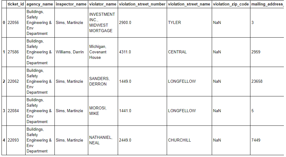
Previewing the data

Initializing function and importing libraries.

def blight_model():
    
    import pandas as pd
    import numpy as np
    import matplotlib.pyplot as plt
    from adspy_shared_utilities import plot_class_regions_for_classifier_subplot
    from sklearn.metrics import roc_curve, auc
    import seaborn as sns
    from sklearn import preprocessing
    from sklearn.model_selection import cross_val_score, accuracy_score, train_test_split
    from sklearn.preprocessing import MinMaxScaler
    from sklearn.model_selection import GridSearchCV

I had to load and preview the datasets to merge them into one to use in our analysis.

    train = pd.read_csv('train.csv', encoding='ISO-8859-1', dtype={'zip_code': str, 'non_us_str_code': str, 'grafitti_status': str, 'violator_name':str, 
                            'mailing_address_str_number': str})

    latlons = pd.read_csv('latlons.csv', encoding='ISO-8859-1')
    address = pd.read_csv('addresses.csv', encoding='ISO-8859-1')
    coord = address.merge(latlons, how='inner', on='address')
    train = train.merge(coord, how='inner', on='ticket_id')

Dropping values and preprocessing data

I initially dropped columns due to potential data leakage.

   dropped = ['balance_due',
           'collection_status',
           'compliance_detail',
           'payment_amount',
           'payment_date',
           'payment_status']
   train.drop(dropped, axis=1, inplace=True)

I dropped string values that I was not likely to encode, except violation code and disposition which I was likely to encode.

    dropstr = [
            'address', 'violator_name', 'zip_code', 'country', 'city',
            'inspector_name', 'violation_street_number', 'violation_street_name',
            'violation_zip_code', 'violation_description',
            'mailing_address_str_number', 'mailing_address_str_name',
            'non_us_str_code', 'agency_name', 'state', #'disposition',
            'ticket_issued_date', 'hearing_date', 'grafitti_status', #'violation_code'
    ]
    train.drop(dropstr, axis=1, inplace=True)

I encoded the violation code and disposition.

    le = preprocessing.LabelEncoder()
    le.fit(train['violation_code'])
    train['violation_code'] = le.transform(train['violation_code'])

    le.fit(train['disposition'])
    train['disposition'] = le.transform(train['disposition'])

I chose a fillna method. (I chose pad after finding it worked with the model better.)

    train = train.fillna(method='pad')

Data analysis and feature selection

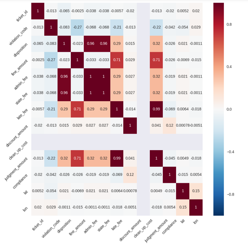
I graphed the correlation between variables.

    plt.figure(figsize=(10,10))
    correlation = train.corr()
    sns.heatmap(correlation, annot=True)
    plt.xticks(rotation=45)
    plt.yticks(rotation=45)

Reviewing the corrrelations, I dropped columns with weak correlations. I kept lat and lon after testing the model and based on common sense that location affects factors that affect compliance.

    moredrop = ['admin_fee', 'state_fee', 'clean_up_cost', 
                #'lon', 'lat'
               ]
    train.drop(moredrop, axis=1, inplace=True)

Preparing data for algorithm testing

I then formatted the training data.

    X = train.loc[:, train.columns != 'compliance']
    y = train.iloc[:,-3]
    y = y.astype(int)

I fitted and transformed the data with Min Max Scaler.

    scaler = MinMaxScaler()
    X = scaler.fit_transform(X)

I split the data into train/test(validation) sets.

    X_train, X_test, y_train, y_test = train_test_split(X,y, random_state=0)

Testing algorithms

I tested different algorithms using the split.

from sklearn.svm import SVC
#from sklearn.naive_bayes import GaussianNB
from sklearn.ensemble import RandomForestClassifier
from sklearn.tree import DecisionTreeClassifier
from sklearn.neighbors import KNeighborsClassifier
from sklearn.linear_model import LogisticRegression
from sklearn.ensemble import GradientBoostingClassifier
from sklearn.model_selection import StratifiedKFold
from sklearn.model_selection import cross_val_score
#from sklearn.ensemble import AdaBoostClassifier

# Create list of models
models = []
models.append(('LR', LogisticRegression(solver='liblinear', multi_class='ovr')))
models.append(('KNN', KNeighborsClassifier()))
models.append(('DTC', DecisionTreeClassifier()))
models.append(('RFC', RandomForestClassifier()))
#models.append(('NB', GaussianNB()))
models.append(('SVM', SVC(gamma='auto')))
models.append(('ADAB', AdaBoostClassifier()))

# Evaluate each model
output = []
names = []
for name, model in models:
    kfold = StratifiedKFold(n_splits=3, random_state=0, shuffle=True)
    cv_results = cross_val_score(model, X_train, y_train, cv=kfold, scoring='accuracy')
    output.append(cv_results)
    names.append(name)
    print('%s: %f (%f)' % (name, cv_results.mean(), cv_results.std()))

LR: 0.924327 (0.000053) KNN: 0.927529 (0.000150) DTC: 0.896116 (0.000915) RFC: 0.930698 (0.000629) NB: 0.928232 (0.000098) SVM: 0.924237 (0.000035) ADAB: 0.933431 (0.000132)

Tuning hyperparameters

Since the ADABoostClassifier had the highest accuracy score, I chose this model. I then tuned the hyperparameters with GridSearchCV.

    clf = AdaBoostClassifier()

    model_params = {
        'learning_rate': [.1,.25,.5,.75,1,1.25,1.5,1.75,2]
    }

    gridsearch = GridSearchCV(clf, model_params)

    model = gridsearch.fit(X_train, y_train)
    model.best_estimator_.get_params()

{‘algorithm’: ‘SAMME.R’, ‘base_estimator’: None, ‘learning_rate’: 0.5, ‘n_estimators’: 50, ‘random_state’: None}

Validating model

A learning rate of .5 yielded the best results so I used it in my classifier and tested on my validation test from my training data to make sure it was still accurate.

    clf = AdaBoostClassifier(learning_rate=.5).fit(X_train, y_train)
    predictions = clf.predict(X_test)
    print(accuracy_score(y_test, predictions))

0.932770826342

Repeat steps with test data

I then repeated the previous steps with the test data and outputted the required format for the autograder.

# Creating test set and merging with geographical data
    X_testset = pd.read_csv('test.csv', encoding='ISO-8859-1', dtype={'zip_code': str, 'non_us_str_code': str, 'grafitti_status': str, 'violator_name':str, 
                        'mailing_address_str_number': str})
    coord = address.merge(latlons, how='inner', on='address')
    X_testset = X_testset.merge(coord, how='inner', on='ticket_id')
    X_testset = X_testset.fillna(method='pad')

# Dropping columns based on correlations from previous analysis
    X_testset.drop(dropstr, axis=1, inplace=True)
    X_testset.drop(moredrop, axis=1, inplace=True)
    
# Preprocessing with the Label Encoder   
    le.fit(X_testset['violation_code'])
    X_testset['violation_code'] = le.transform(X_testset['violation_code'])
    le.fit(X_testset['disposition'])
    X_testset['disposition'] = le.transform(X_testset['disposition'])

# Finalizing with the MinMax Scaler
    X_testsetfinal = scaler.fit_transform(X_testset)

# Calculating probabilities and putting into form specified for autograder
    test_pred = clf.predict_proba(X_testsetfinal)[:,1]
    ans = pd.DataFrame(test_pred,index=X_testset.ticket_id.values, columns=['Probability'])
    ans.index.name = 'ticket_id'    
    return ans

The resulting AUC was 0.788964207005 which achieved full marks (passing was 0.7, full marks was 0.75).